Path loss constant and RSSI distribution

Path loss model

The power loss of a signal is a function of the distance.

is a constant signal propagation exponent that is specific to the testing environment. is a RSSI value taken at distance . Setting to 1 removes the fraction and thus assumes the RSSI value at 1m.

The measurement data is available at https://gitlab.com/mark-matura/ble-ips-files/-/tree/master/RSSI_measurements/05-10_path_loss_parameters.

Average RSSI at varying

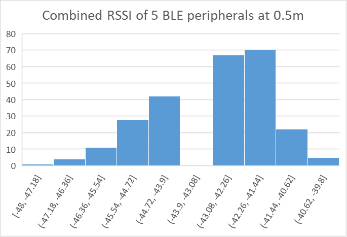
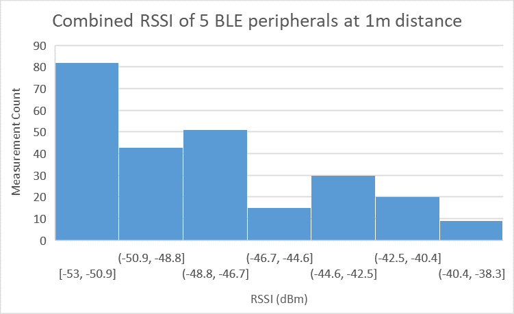
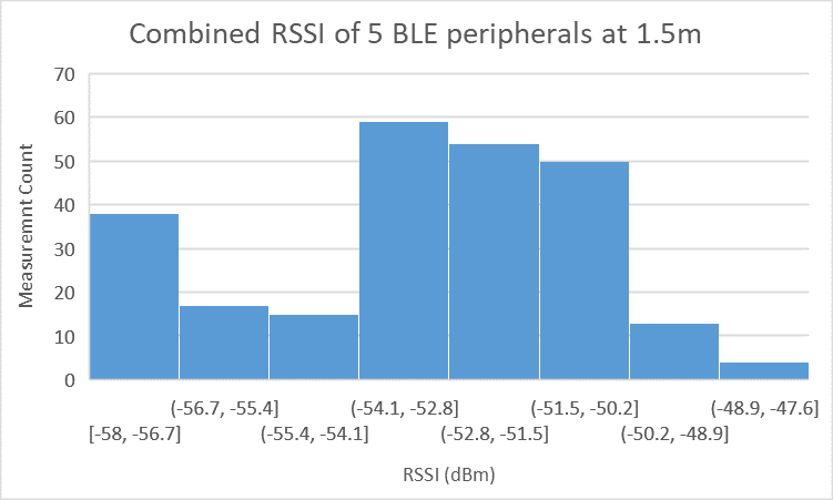
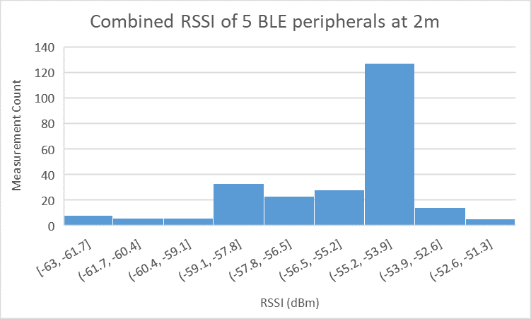
Distance (m)	0.5	1	1.5	2	2.5	3	4
Average RSSI (dBm)	-43.092	-47.916	-53.212	-55.812	-57.476	-60.776	-62.036
Standard Deviation RSSI (dBm)	1.47657	3.741247	2.3317	2.25321	1.689034	1.778335	1.705973

The standard deviation is not bad for the averages but is subject to larger fluctuations with certain devices.

Least squares based regression

I ran these numbers through GnuPlot to pass the data through some linear regression.

degrees of freedom    (FIT_NDF)                        : 6
rms of residuals      (FIT_STDFIT) = sqrt(WSSR/ndf)    : 1.25371
variance of residuals (reduced chisquare) = WSSR/ndf   : 1.57178

Final set of parameters            Asymptotic Standard Error
=======================            ==========================
n               = 2.41514          +/- 0.1279       (5.296%)

According to GPL the signal propagation exponent of my living room is based on averages of 350 measurements and linear regression. It remains to be seen how accurate this is.

According to Wikipedia it is comparable to an office with a soft partition at a signal frequency of 1.9GHz.

Curve fit of in respect to where is -47.916 dBm and is 2.41514.

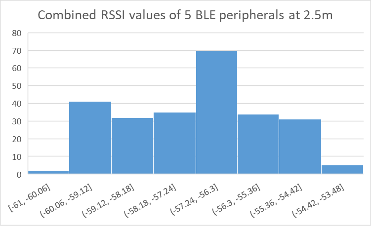
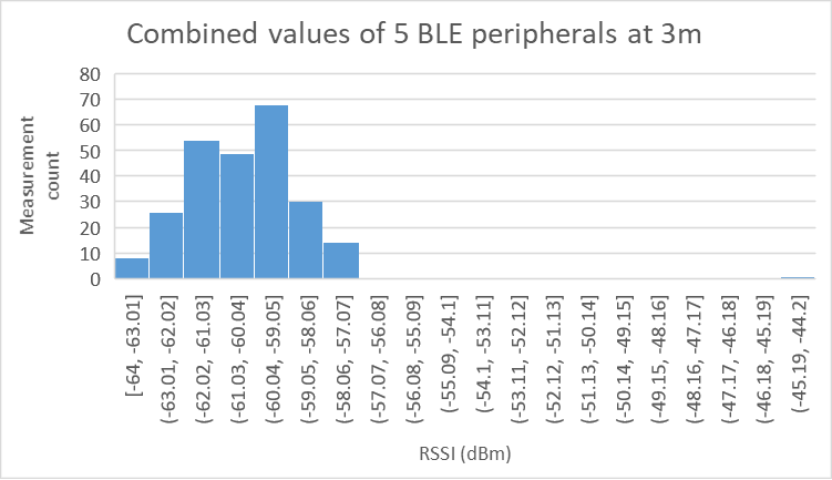
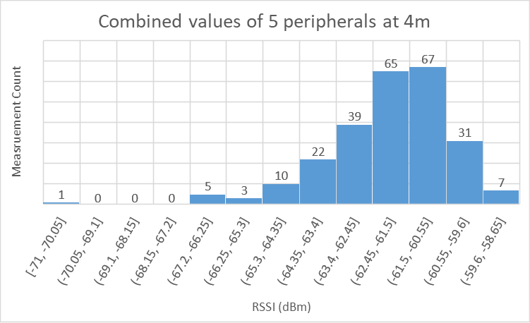
Distribution of RSSI measurements (Histograms)

The distributions seem to be of gaussian form. That is nice, since the kalman filters described in 05-10 noise reduction are valid.